
Authors: The Nubank Experimentation Platform’s Data Science team is Abel Borges, Brando Morais, Luís Assunção, Paulo Rossi, Ramon Vilarino (in alphabetical order).
No feature in the platform would be possible without the support of the entire squad — a special thanks to Thiago Nunes (PM), Thiago Parreiras (Product lead), and Miguel Bitarello (Engineering lead).
Introduction
A/B testing is a cornerstone of product development at Nubank, allowing us to make data-informed decisions by comparing different versions of a product or feature to see which performs better. This rigorous approach ensures that every change we implement is backed by empirical evidence, leading to continuous improvement and a superior user experience.
However, a persistent challenge in experimentation is the issue of experiment sensitivity. Often, the effects we aim to measure are subtle or small, making them difficult to detect with statistical significance. This limitation can hinder our ability to identify changes and optimize our products effectively. To overcome this, our team embarked on a journey to explore advanced variance reduction techniques to improve statistical power.
Improving statistical power translates directly into increased precision for our estimates, thus reducing the duration of experiments. This allows for faster and safer iteration.
Among the approaches we investigated, “Controlled-Experiment using Pre-Experiment Data” (CUPED) stood out. CUPED is a statistical method that leverages pre-experiment data to reduce the variability of key metrics. By accounting for baseline differences among experimental units, CUPED can significantly improve the statistical power of our experiments, making it easier to detect even smaller, yet meaningful, effects.
This article shares the 3 key lessons we learned from the challenging yet rewarding process of implementing CUPED within Nubank’s robust experimentation platform. These insights offer valuable guidance for any organization looking to enhance precision and efficiency when scaling their A/B testing efforts.
Check our job opportunities
Background
CUPED was first introduced by Microsoft researchers Deng and others (2013) and has been widely used in companies such as Netflix, Booking, Eppo, Walmart, and many others. Notes by other researchers (Lin (2013), Deng and Hu (2015), Deng and others (2023)) highlight the relationship of CUPED to linear regression, and how different assumptions in CUPED map to different regression specifications.
Suppose that our experiment has a target metric Y which is calculated using all events for a given customer after they are exposed to the experiment. We’re interested in estimating the Average Treatment Effect (ATE), so we calculate the difference in means between treatment and control,

where Δ is an unbiased estimator of the ATE. Assume we’re able to compute a covariate X using events that occurred prior to the customer’s exposure to the experiment. With that, we can write

where θ is a scalar parameter. Since subjects were randomly assigned between control and treatment groups, E(Xt) -E(Xc)= 0 and thus , Δadjusted is also an unbiased estimator of the ATE.
The goal is to choose a value for θ that reduces the variance of Δadjusted result as much as possible. Using the expression for the variance of the linear combination of two random variables, we can expand the variance for Δadjusted:

By setting its first derivative to zero, we can determine the optimal value, θ*, that minimizes this variance:

And finally we have:

A natural choice for X are pre-exposure measurements of Y; for instance, key transactional metrics for a bank usually present strong serial correlation (i.e. correlation of the metric with itself in the past). However, this demonstration applies to any covariate.
Notice that if we write θ* in terms of the covariances between unit observations rather than between averages, then we can write:

where θc=Cov(Xc,,Yc) / Var(Xc) and θt=Cov(Xt,,Yt)/Var(Xt). In other words, it is a weighted average from two θ parameters of each group in terms of their sample variances.
Note that θc and θt are coefficients of a simple linear regressions per group, and θ* is a combination of both. Further details can be found in Lin, Section 2 (or 3).
Lesson 1: Be aware of unequal variants.
When control and treatment groups are equally sized, θ* can be approximated from pooled statistics, as described in Deng et al. (2013):

which yields Δpooled. However when the experiment groups have different sample sizes (nc π nt) and the treatment changes the serial correlation of the metric (Cov(Xc,Yc) ≠ Cov(Xt,Yt) ), the variance of Δpooled can be larger than the variance of the naive estimator Δ.
When simulating scenarios with highly unequal groups (90%/10% split) and a treatment group’s covariance three times larger than control’s, the ATE distributions demonstrate reduced efficiency with a pooled estimation, as illustrated in the plot below.

At Nubank, we had originally implemented CUPED by estimating θpooledfor each variant pair for every experiment. However, we run multiple experiments that violate the assumptions of this original estimator. Lin (2013) showed that *Δadjusted is at least as efficient as both Δ and Δ pooled. Following their conclusions, we assessed whether this change would be meaningful for our metrics and decided to change our implementation to use θ*. Though seemingly minor, this change significantly enhanced the robustness and precision of our analyses, leading to more dependable experimental conclusions.
Lesson 2: How We Defined a Standard 42-Day Lookback Window
Following the decomposition of θ* as a weighted sum of θ-like coefficients within each group, the variance of Δ*adjusted can be recast as a function of the metric standard deviations and serial correlations (pt, pc) between its post and pre-exposure versions, π ∈ (0,1) being the sampling rate of the treatment group:

Note that the higher the correlation between post-exposure and pre-exposure metrics in absolute terms, the higher the variance reduction. As noted in the background section, a straightforward method is to set X equal to Y in the past, which naturally leads to using the same variable as the control variate during the pre-experiment observation window. However, this raises the question: How can we determine the optimal pre-experiment metric aggregation period for CUPED?
Nubank offers a diverse portfolio of products and services, ranging from its foundational credit card offerings to its expanding shopping marketplace. Given this inherent diversity, each product operates within its own distinct market and targets a different segment to the customer base. For example, the seasonality of a user searching for flights in our marketplace is very different from those investing in crypto assets.
Ideally, each metric and experiment would have its own pre-experiment window. However, this level of flexibility and implementation overhead is not currently feasible in our platform. Therefore, we chose a generic window that would adequately capture most past user behavior without significantly increasing pipeline costs.
For that, we ran several simulations, sampling subjects from our experiments with varying sample sizes and durations. This approach allowed us to incorporate simulated data with real treatment effects to obtain the optimal window. Our analysis concentrated on time windows that were precise multiples of seven, capturing and addressing the weekly patterns present in the data.
The average variance reduction results, presented as a function of the lookback window, are detailed below.

We selected a fixed 42-day lookback window for our analysis due to its balanced performance across all metrics and experiments. This timeframe presented a good trade-off between minimized variance while managing the computational costs of our metric pipeline. We also found that a 42-day window is good enough to capture average business dynamics, particularly encompassing at least one credit card billing cycle, ensuring a comprehensive view of customer behavior and financial activity.
However, the actual impact of CUPED varies significantly across our diverse ecosystem. The chart below illustrates the distribution of variance reduction we observed in practice over hundreds of metrics in thousands of different experiment comparisons.

This distribution reveals a couple of key insights:
- About 40% of comparisons had their variance reduced by more than 20%. In rare instances of specific populations and metrics, variance was reduced by almost 99%.
- In about 12% of comparisons, there was no pre-experiment data available (NA). In the remaining cases, variance was reduced by less than 10%.
Ultimately, this shows that while finding a perfect, one-size-fits-all lookback window is challenging, our standardized 42-day period provides a meaningful reduction in variance for a vast majority of our metrics. It’s a challenge to find good, generic variance explainers.
Lesson 3: The shrinkage effect
The path to fully integrating CUPED wasn’t just a technical one. One of the primary reasons we initially hesitated to make it the default view in our experimentation platform was the shift in how the Average Treatment Effect (ATE) is interpreted. Although the new estimator is more precise, its point estimate also changes and it can significantly differ from the raw, unadjusted lift our teams were accustomed to.
This discrepancy is further complicated by our use of relative lift as the primary result in the platform, calculated as the ATE divided by the sample mean of the control group.

Explaining a metric that combines an adjusted numerator with an unadjusted denominator adds another layer of complexity. This required a significant investment in training and office-hours with our users and stakeholders to ensure that they understood not just that the results were more accurate, but why. This effort was crucial to build trust and prevent misinterpretation of the adjusted outcomes.
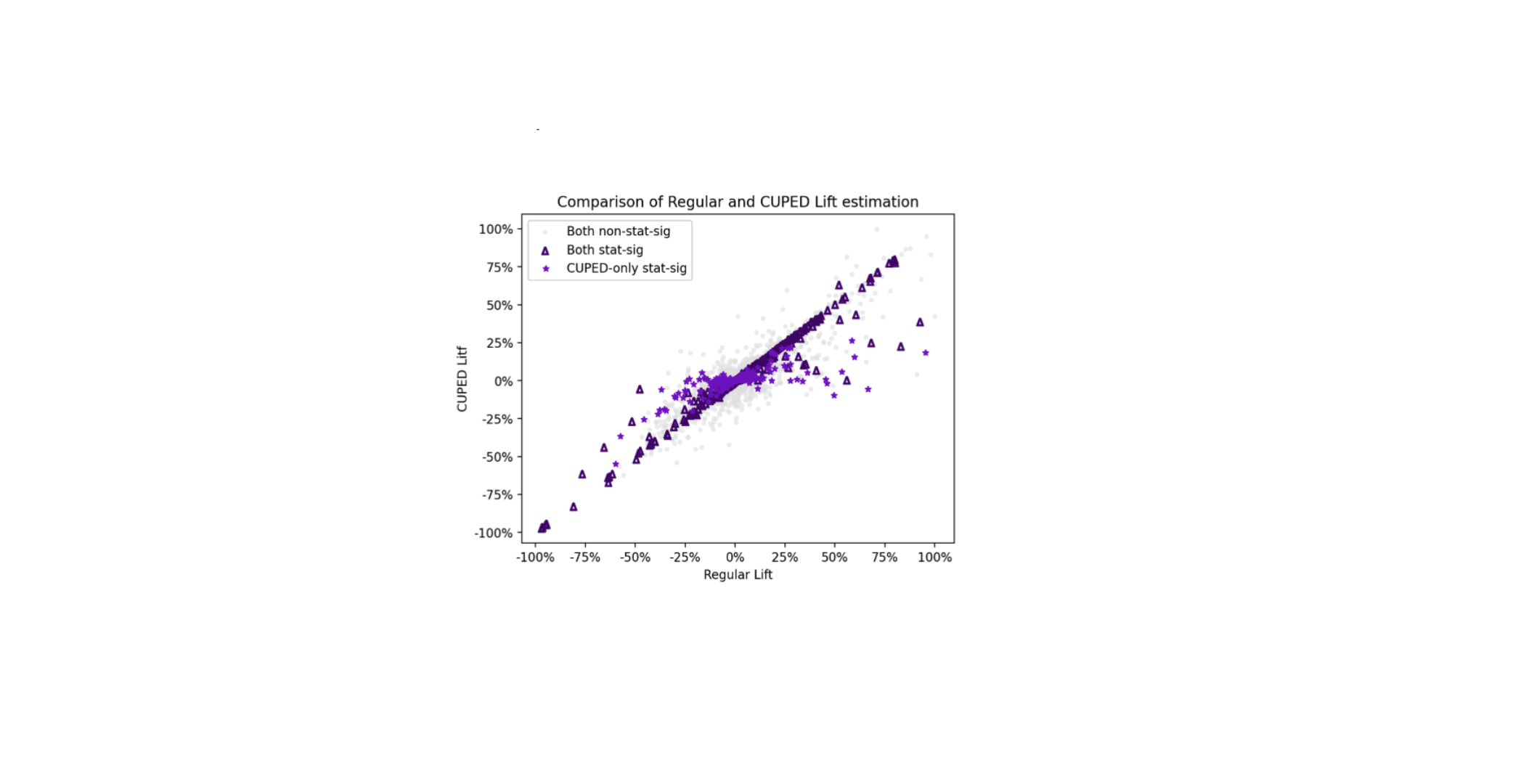
The following scatter plot compares the relative lift estimated by our standard analysis (“Regular Lift”) against the relative lift estimated using CUPED (“CUPED Lift”) across thousands of experiments and over hundreds of binary and continuous metrics.

The chart reveals three key insights. First, the dense cluster of points is symmetric around the y=x line. This empirical observation aligns with the theory that the CUPED-adjusted lift remains an unbiased estimator.
Second, light purple stars represent experiments where the standard analysis failed to find a statistically significant result, but the CUPED-adjusted analysis succeeded. Although statistical significance is an arbitrary definition (and we apply some conservative corrections like Bonferroni in our multiple-metric dashboards), these points might represent “hidden wins” and “missed warnings”, uncovered due to CUPED’s ability to increase statistical power. Third, a closer look at these points also reveals a subtle but important “shrinkage effect”: the CUPED lift for these blue stars is often closer to zero than the estimate from the regular analysis. This shrinkage is not a weakness but a crucial feature that helps mitigate Type M (magnitude) errors. By attaining a higher power for experiments originally dimensioned for the naive estimator, CUPED shrinks the point estimate towards the true treatment effect in statistically significant comparisons. . These shrinked estimates are illustrated as dark purple triangles in the chart.
Conclusion
Nubank’s implementation of CUPED on its Experimentation Platform yielded 3 significant insights. First, it’s crucial to be aware of unequal variances and sample sizes between control and treatment groups, as using a pooled estimator for theta (θpooled) can decrease precision, especially when the treatment changes the serial covariance of the metric. The company switched to a more robust weighted average estimator (θ*) to address this, which improved the accuracy of their analysis.
Second, a standard 42-day lookback window was chosen as a practical trade-off. While the optimal pre-experiment data period varies with different metrics and experiment scenarios, this fixed window was found to effectively reduce variance for the majority of metrics while being computationally efficient.
Lastly, we observed a shrinkage effect where CUPED-adjusted lifts for statistically significant results are often closer to zero than the regular analysis. This is a valuable feature that helps mitigate Type M errors by correcting for overestimated effects and provides a more precise and realistic estimate.
Building on the success of CUPED, we are actively exploring new avenues for variance reduction. This includes investigating the incorporation of additional covariates and developing robust methodologies to platformize advanced variance reduction techniques at scale across all our experimentation efforts. Our ongoing work in this area reinforces Nubank’s commitment to leveraging sophisticated experimentation methods, ultimately supporting our mission to continuously make better product decisions that benefit our customers.
Bonus lesson
Implementing CUPED for Ratio Metrics
Given a ratio metric R = Y / Z, Var(R) can be estimated using the Delta Method theorem. This statistical approach is particularly useful for approximating the variance of functions of normal random variables. As detailed in Sections 2.2 and 3.2 of the paper by Nie et al. 2020 paper and in the formula below:

where n is the sample size. The most interesting challenge of this implementation lies in accurately determining the covariance of a ratio metric for calculating θ* .
Consider two ratio metrics: Y/Z as the post-experiment metric and X/W as the pre-experiment metric. A first-order approximation for the covariance of two ratio metrics can be derived after linearization via Taylor expansion:

With the covariance between pre- and post-experiment ratio metrics calculated, the ATE and its variance can be estimated using the exact same procedure described in the introduction.
Check our job opportunities


Great breakdown of Nubank’s CUPED implementation! At TheSoftReview, we also explore advanced SaaS tools and analytics techniques, and it’s insightful to see how variance reduction can significantly improve experiment precision in real-world platforms.
This is great! Very informative.