
most read
Software Engineering
Why We Killed Our End-to-End Test Suite Sep 24
Culture & Values
The Spark Of Our Foundation: a letter from our founders Dec 9
Software Engineering
The value of canonicity Oct 30
Careers
We bring together great minds from diverse backgrounds who enable discussion and debate and enhance problem-solving.
Learn more about our careers


Author: Fabio Souza
At Nubank, we are constantly pushing the boundaries of how Artificial Intelligence can help us better understand our customers’ financial journeys. Our previous posts have detailed how we leverage transformer-based foundation models to convert sequences of transaction data into powerful embeddings, enabling us to better meet the financial needs of our customers at the right time [1, 4]. We have explored the interface that translates raw transaction data into embeddings that our models can understand [2], discussed the nuances of fine-tuning these models for specific tasks [3], and demonstrated how we optimize user narratives by thoughtfully selecting and representing transaction features and sources [5].
However, the aforementioned journey of optimizing user narratives is continuous. As we highlighted in our previous posts, choosing which information from a transaction to include and how to represent it matters, especially given the limited context length of our transformer architectures. Today, we dive deeper into a crucial aspect of transaction data: the timestamp of when the transaction happened. How we encode the “when” of a transaction can significantly impact a foundation model’s ability to understand a customer’s financial state and predict future behaviors.
In the remainder of this blog post, we first discuss the challenges with using absolute timestamps. Then, we propose a different approach that uses time deltas to represent the time information, detailing the design process and key decisions. Lastly, we present the experimental design and results that validate this new approach on a real business problem.
The Challenge with Absolute Timestamps
Initially, when representing transactions, our token-level models encoded absolute timestamps represented by special tokens for <MONTH>, <DAY>, and <WEEKDAY> for each transaction. While straightforward, this approach presented several challenges for a foundation model designed to build user representations potentially spanning long periods of time. The figure below reiterates the existing transaction tokenization procedure used by our models [2,4].
For example, consider a scenario where a customer becomes inactive for an extended period, perhaps a year, and then resumes activity. If the model solely relies on absolute timestamps, the embeddings generated at any point during this inactivity period would remain identical. More specifically, the model lacks a “notion of now”. This insensitivity to inactivity periods means the embeddings might not accurately reflect the customer’s current behavior, which is an aspect inherently captured by traditional machine learning features that are calculated over time windows relative to a “score date” (e.g., 1 month, 3 months, 6 months).
Furthermore, absolute timestamp encodings can lead to models overfitting to specific date periods or combinations of <MONTH><DAY><WEEKDAY> and other transaction attributes, especially if the training data covers less than a full year, or if the target has strong seasonalities. This limits the model’s ability to generalize effectively during inference, particularly for out-of-time (OOT) data.
Check our job opportunities
Introducing Time Deltas: A Relative Approach
To address the limitations of absolute time encodings, we hypothesized that representing the timestamp information as a “time delta,” or the “age” of the transaction relative to the score date (the “now”), would be more effective. This approach allows embeddings to reflect periods of inactivity and better capture the recency and relevance of past transactions.
As with other transaction features, we implemented this by designing a special token. More specifically, we implemented this by quantizing time deltas into distinct buckets, similar to how we handle transaction amounts. These buckets are then represented by their own special tokens, such as:
Importantly, there are two hyperparameters we must choose. Firstly, the granularity/scale of the time deltas must be selected. Secondly, we must define a threshold where time deltas are truncated. In the above example, the time delta truncation threshold was set to two years. Therefore, in this case, any transaction that is greater than two years from the score date is truncated to: <TIMEDELTA:ABOVE-2-YEARS>. In the following section, we explore setting these parameters by analysing the distribution of time deltas in our data.
Defining the Time Delta Horizon and Granularity
As mentioned, an important step to effectively use the time delta special tokens is sensibly defining the maximum time delta truncation threshold. For example, selecting a cap that’s too small risks losing valuable information. Conversely, an overly large cap can introduce an excessive number of special tokens, which may be undertrained if their occurrence is rare during the training phase.
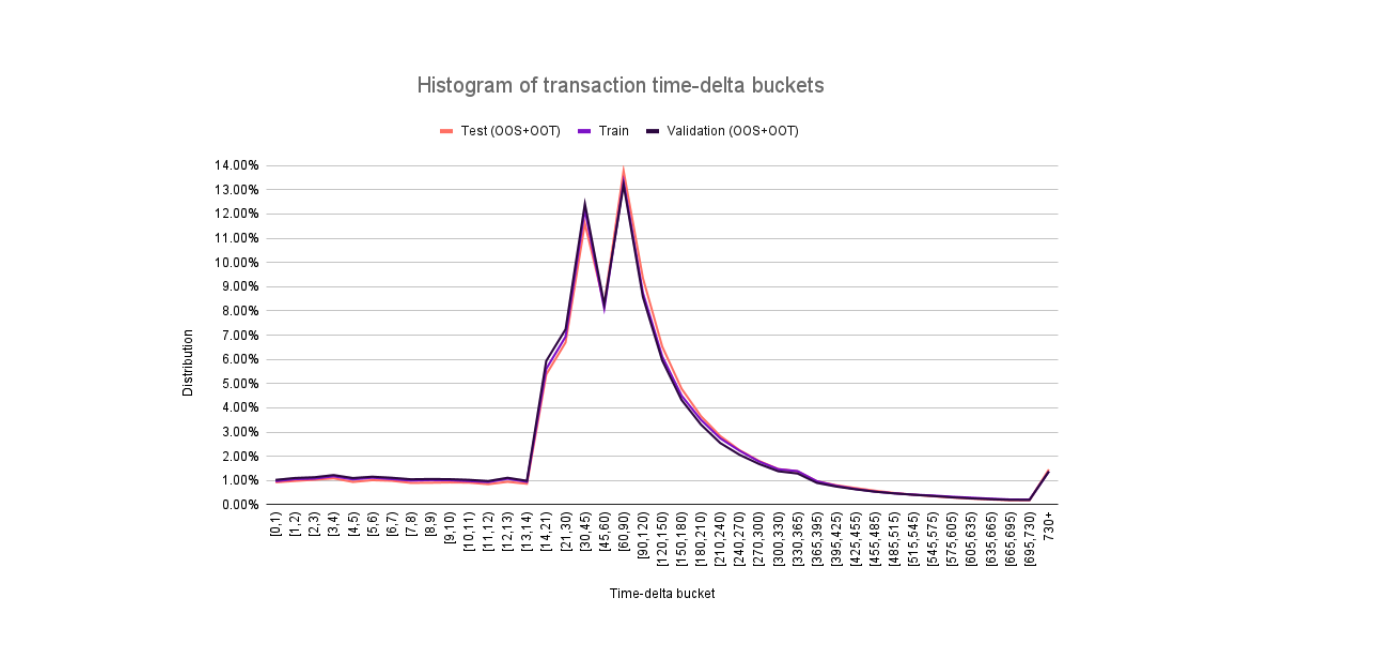
By plotting the cumulative distribution of transaction temporal window sizes (the time between the oldest and most recent transactions in a sequence) for our training dataset, we observed that nearly 97% sequences contained transactions up to two years old. Based on this, we decided to start by using two years as the time delta cap for our encoding. Next, we need to choose a granularity for the time delta buckets. We experimented with two different bucket strategies:
Using the default strategy, we plotted the histogram of the time-delta buckets comparing the distributions on the train, validation and test datasets. We can see that the distributions are consistent for the 3 dataset splits, which is a positive sign for generalization in the out-of-time period. The less granular strategy has a similar distribution.
Experimental Design and Results
To rigorously test our hypothesis that a relative time representation is better than an absolute one, we pre-trained four foundation model variants on the same dataset using the next token prediction task. Then, we fine-tuned each foundation model variant on a downstream task using a labeled dataset for a business problem. The variants were:
1. Baseline: Uses DAY, MONTH, WEEKDAY special tokens for absolute timestamp encoding.
2. Relative Time-Delta (REL): Uses only the relative time-delta encoding with the default bucket strategy.
3. Relative Time-Delta, Less Granular (REL-LOW): Uses only the relative encoding with the less granular bucket strategy.
4. Relative Time-Delta + Absolute Encoding (REL+ABS): Combines the relative time-delta with the baseline’s absolute encoding.
To make the distinction between these variants clear, we will explore an example of how each encodes a set of transactions. Let’s consider a user who has the following 4 transactions (with date, description and value):
Then, using a score date of 31/08/2025 00:00:00 AM, we would get the following tokens for the time representations:
After pre-training and fine-tuning each of the variants, we evaluated the four models on a test set containing data from a later time period, which more accurately reflects real-world production performance. The primary metric for evaluation was AUC. The Figure below shows the delta AUC versus the baseline variant.
Key Takeaways:
In this work, we found that how we represent the temporal information can significantly impact the foundation model’s ability to understand customer financial behavior. Encoding time as time deltas instead of absolute dates improved ROC-AUC by 0.2 percentage points (pp), while simultaneously reducing the number of tokens per transaction by about 15%, enabling longer transaction histories within the same token budget. These findings highlight a key principle: the way we design our data representation can have a substantial impact on model performance. The weaker results of the less granular time delta setting further underscore the importance of systematic experimentation and evaluation to achieve optimal results.
References
[1] Braithwaite, D., & Udagawa, H. (2025, March 24). Understanding our customers’ finances through foundation models. Building Nubank. https://building.nubank.com/understanding-our-customers-finances-through-foundation-models/
[2] Braithwaite, D., & Udagawa, H. (2025, April 22). Defining an interface between transaction data and foundation models. Building Nubank. https://building.nubank.com/defining-an-interface-between-transaction-data-and-foundation-models/
[3] Braithwaite, D., Cavalcanti, M., & Udagawa, H. (2025, May 14). Fine-tuning transaction user models. Building Nubank. https://building.nubank.com/fine-tuning-transaction-user-models/
[4] Braithwaite, D. T., Cavalcanti, M., McEver, R. A., et al (2025). Your Spending Needs Attention: Modeling Financial Habits with Transformers. arXiv preprint arXiv:2507.23267.
[5] Foust, T. (2025, July 29). Optimizing user narratives for foundation models. Building Nubank. https://building.nubank.com/optimizing-user-narratives-for-foundation-models/
Check our job opportunities